Open-Vocabulary Wildlife Detector from aerial images
leveraging textual inputs for open vocabulary animal detection
Highlights
- Developed OpenWildlife (OW), an innovative open-vocabulary multi-species wildlife detector capable of identifying species across terrestrial and marine environments using natural language inputs
- The model is trained on 20 geographically diverse datasets, including birds from multiple continents, pinnipeds, cetaceans, wild animals from Africa, and domestic livestock
- Achieved state-of-the-art performance across 20 datasets with detection performance upto 0.981 mAP50 in fine-tuning setting and good generalization across 6 datasets in zero-shot setting with upto 0.812 mAP50
- Developed a novel search that uses k-nearest neighbors and breadth-first search to locate areas with high probabilities of social species presence. Our search method captures 98.7% of species while exploring only 32.3% of the total images
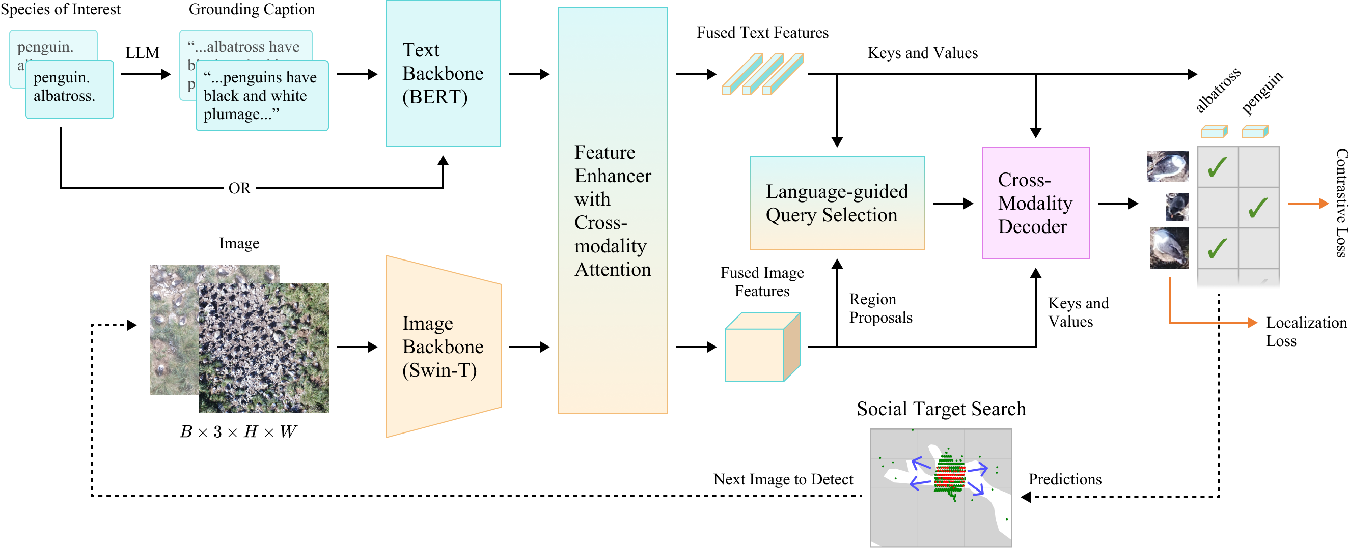
Dataset
We consolidated all publicly available aerial wildlife datasets for our study. Each dataset was preprocessed into the COCO annotation format with bounding boxes; datasets containing only key points were converted into fixed-size bounding boxes. The collected datasets encompass various species, including birds from multiple continents, pinnipeds, cetaceans, wild animals from Africa, and domestic livestock. Detailed descriptions of individual datasets are provided in the supplementary material.
The 26 datasets were partitioned into two groups: 20 were used for open-set continuous pretraining, while 6 were reserved for zero-shot evaluation. This division was designed to assess the model’s adaptability across geographically-diverse contexts, such as tundras, tropical oceans, and deserts.
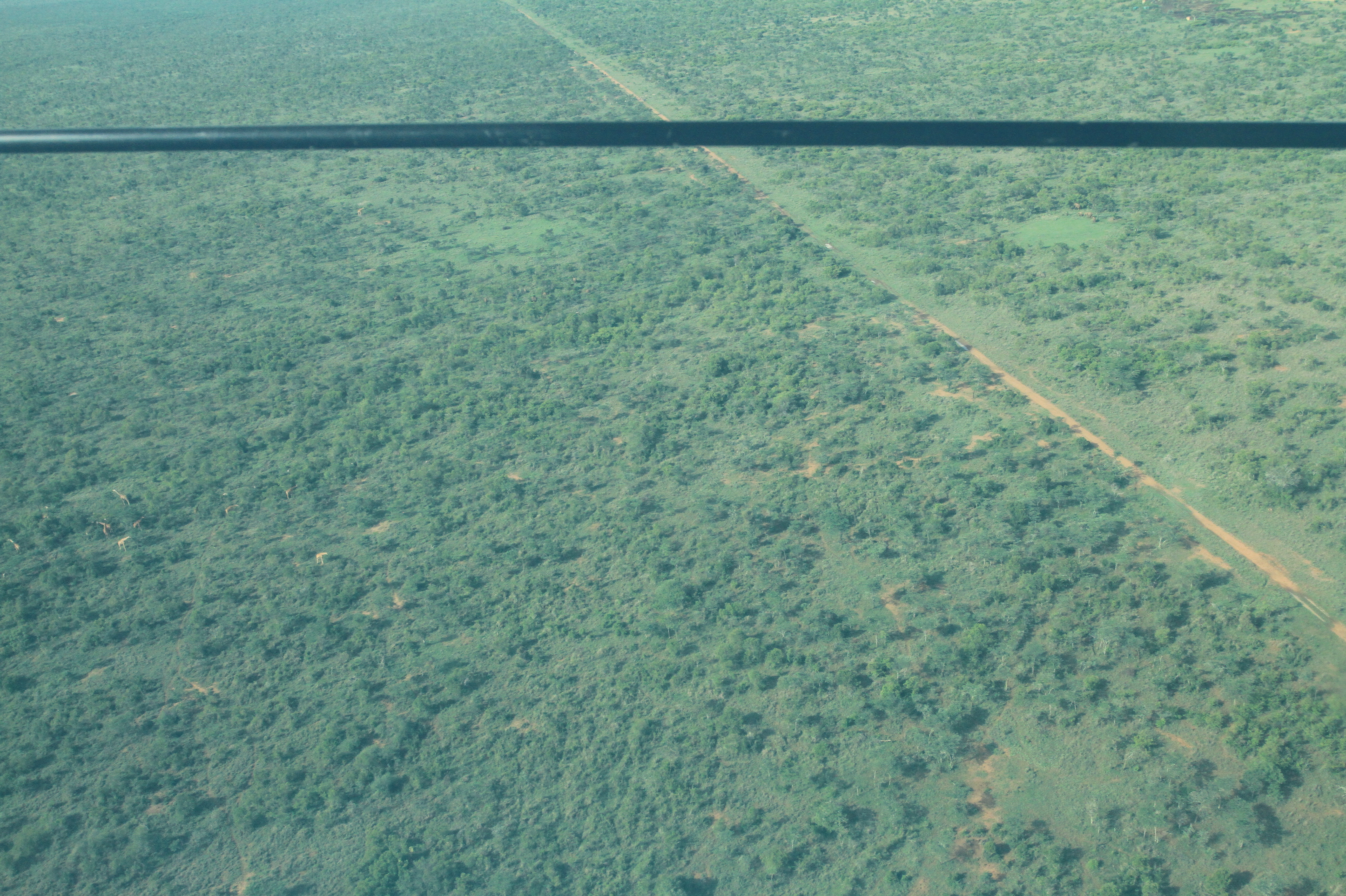
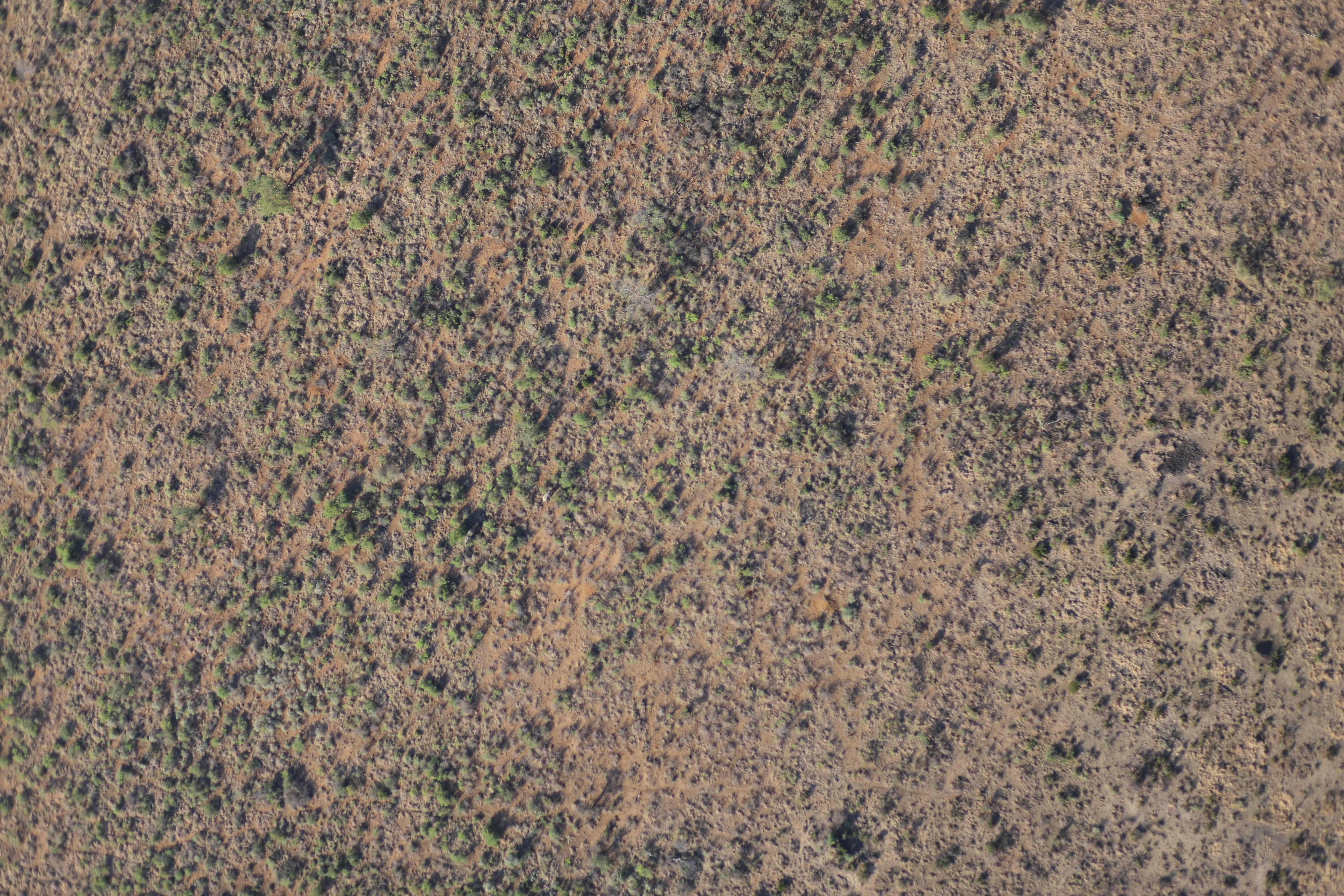
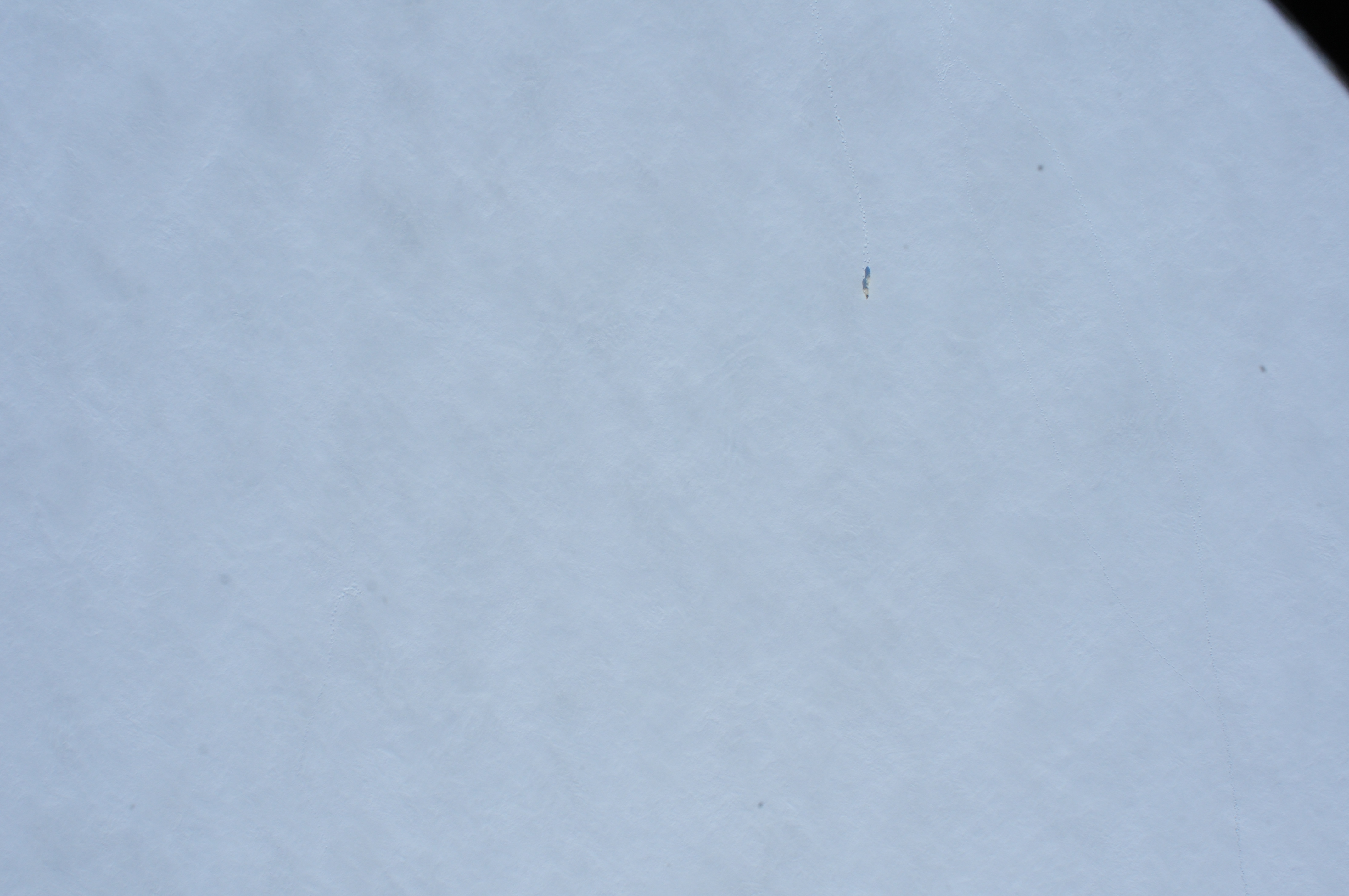
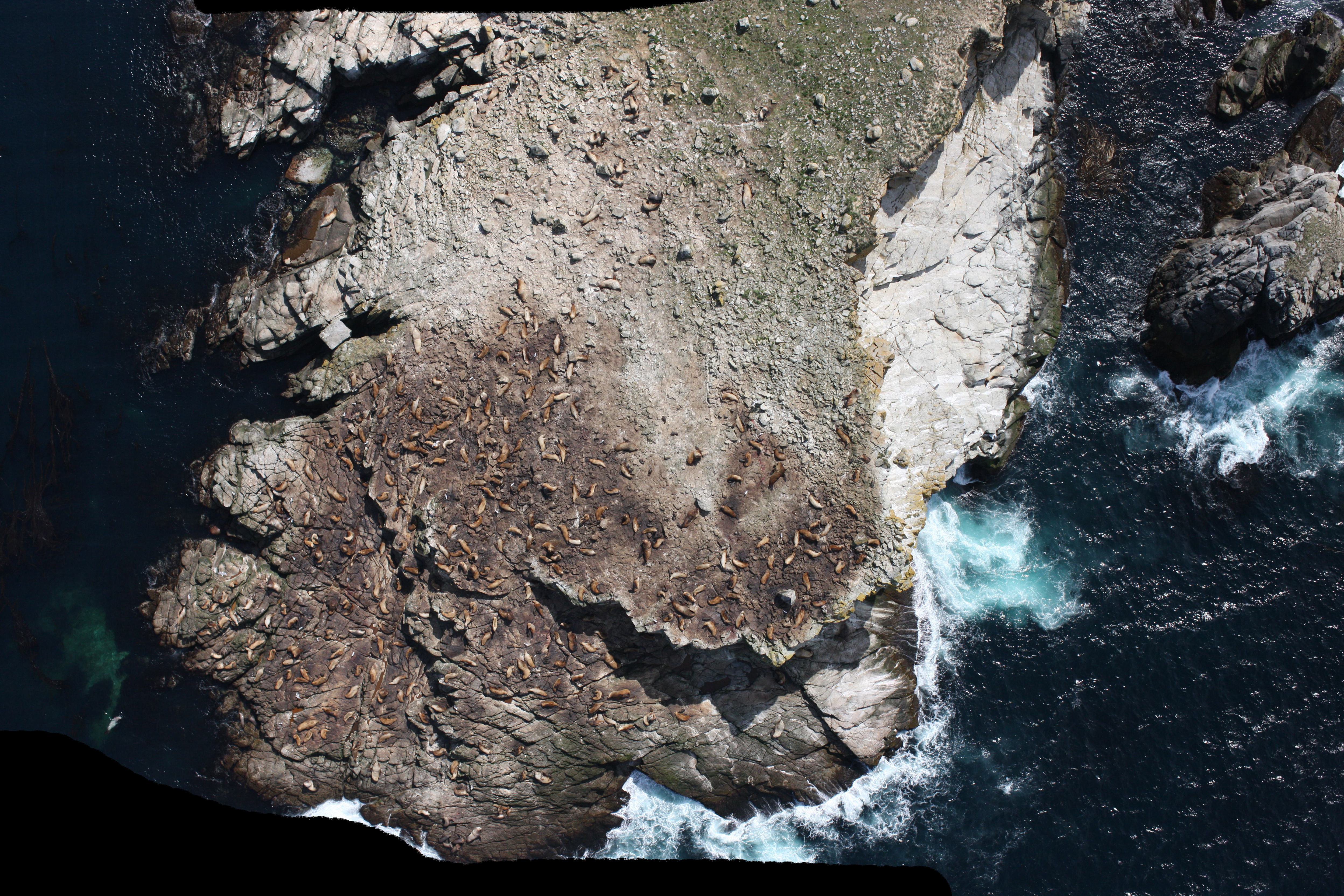

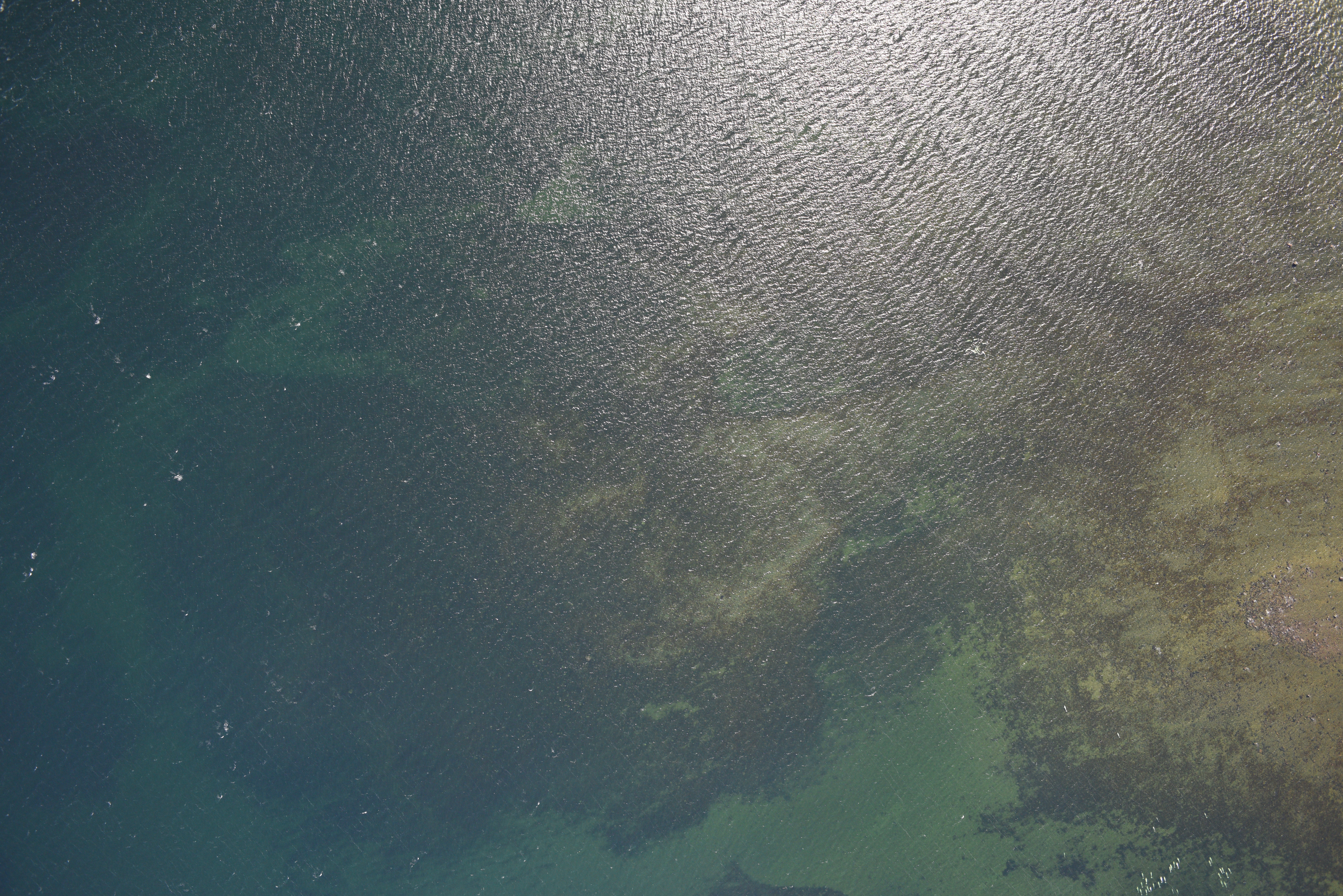
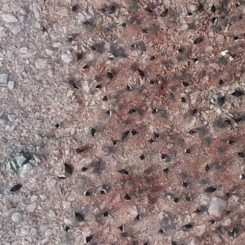
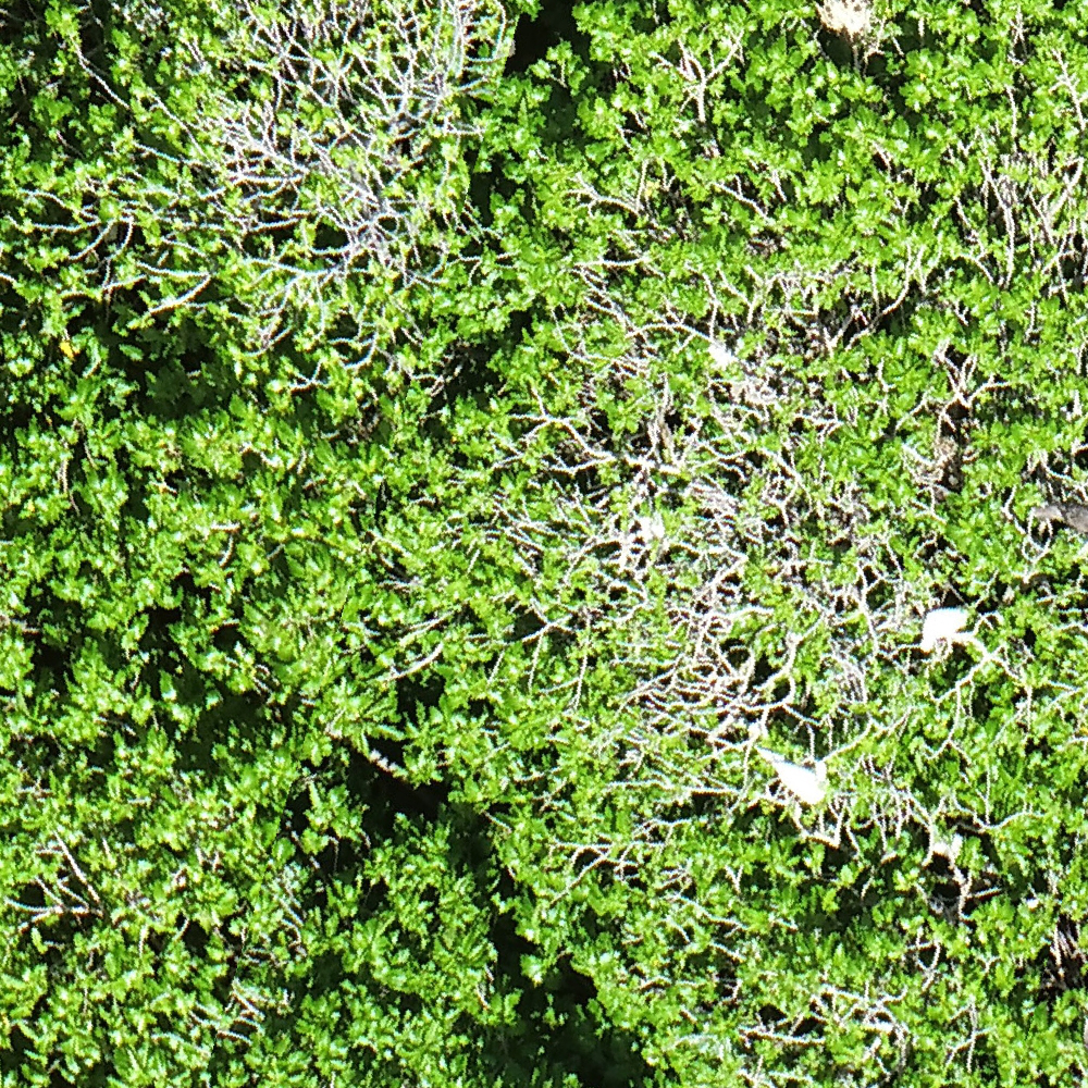
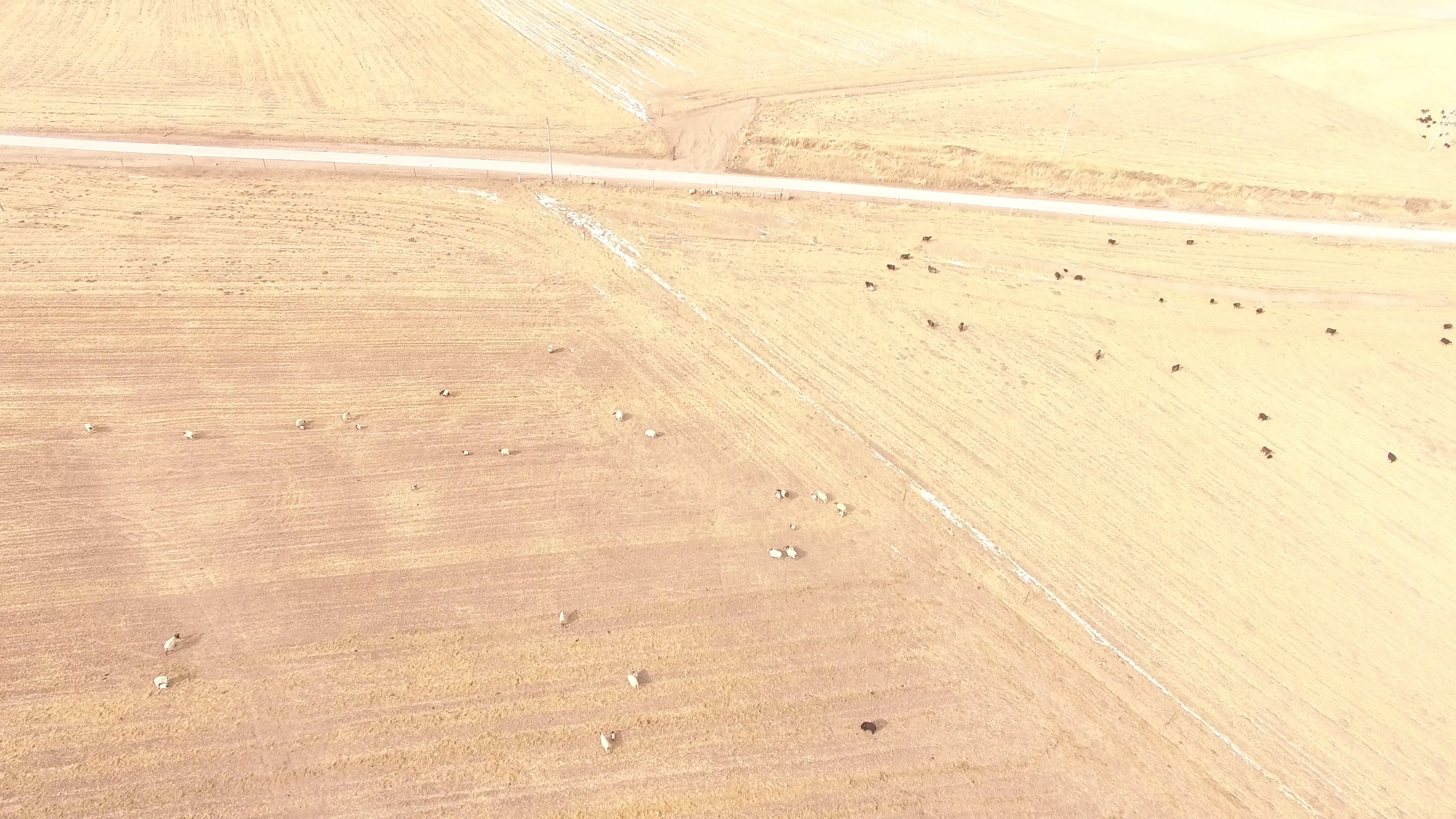
The above images shows the prediction capabilities of OpenWildlife across diverse terrain and species.In some cases, the model produces additional bounding boxes, which appear valid and may highlight potential labeling errors in the dataset. Click on individual images to zoom in. Use the toggle button to switch between predictions and original images. Box color coding; TP: Green, FP: Red, FN: Blue.
Caption generation
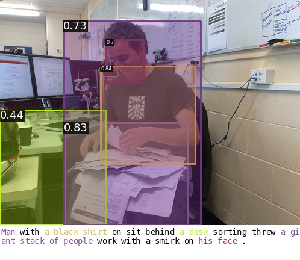
Example of rich annotation in general computer vision datasets.
In general computer vision there are datasets like O365, GOLD and V3Det which have rich semantic annotation for each image. An example of such rich annotation is shown in the figure below. However in aerial images of animal, obtaining such rich annotation is difficult and laborious. To circumvent that, we leverage the world knowledge acquired by LLMs. Specifically, we use OpenAI’s GPT-4o-mini, Batch API to generate a caption for our image with three components: a general description of the dataset, visual description of the animal present and details about their habitat and population density. These captions provides the necessary context that will help improve the prediction performance.
An example of ChatGPT generated annotation for aerial imagery is shown in the figure below.
Generated Caption: An aerial view over Cumberland Sound Bay, Nunavut, in 2014. Possible species present include beluga whales. Beluga whales are easily recognizable by their white coloration and rounded foreheads, often referred to as ”canaries of the sea” due to their vocalizations. These social species tend to form pods, with population densities often ranging from a few individuals to several dozen in a given area, especially in feeding grounds.
Result
The table below presents the mAP50 performance of the OpenWildlife model across various datasets during open-set continuous fine-tuning. In this setup, the model has been exposed to the domain and species during training but is evaluated on a separate, held-out test dataset to assess its performance.
| Dataset | Literature Results | OW Keyword | |
|---|---|---|---|
| Lit. Metric | mAP50 | ||
| Michigan | 0.73 F1 [70] | 0.83 F1 | 0.831 |
| IndOcean | 0.76 F1 [70] | 0.81 F1 | 0.845 |
| NewMex | 0.76 F1 [70] | 0.80 F1 | 0.712 |
| Palmyra | 0.80 F1 [70] | 0.68 F1 | 0.709 |
| Pfeifer | 0.66 F1 [70] | 0.86 F1 | 0.848 |
| Seabird | 0.69 F1 [70] | 0.93 F1 | 0.957 |
| WAfrica | 0.62 F1 [33] | 0.63 F1 | 0.544 |
| Turtle | 0.27 F1 [21] | 0.38 F1 | 0.247 |
| ArctSeal | 0.87 F1 [19] | 0.87 F1 | 0.921 |
| Han | 0.89 mAP50 [24] | 0.97 mAP50 | 0.969 |
| WAID | 0.98 mAP50 [46] | 0.98 mAP50 | 0.981 |
| Kenya | 0.77 mAP30 [15] | 0.86 mAP30 | 0.849 |
| AED | 0.89 mAP † [47] | 0.90 mAP † | 0.856 |
| Sea Lion | 10.86 RMSE [29] | 10.84 RMSE | 0.705 |
| Penguin | 39.4 RMSE [55] | 365.68 RMSE | 0.404 |
| Izembek[71] | - | 0.391 | |
| DFOW14 | - | - | 0.761 |
| DFOW15 | - | - | 0.791 |
| DFOW16 | - | - | 0.750 |
Results of open-set continuous fine-tuning. Bold numbers denote the best metric between literature results and OW Keyword results. Results marked with † indicate a 200-pixel Chebyshev distance allowance to be considered a true positive.
The primary objective of the OpenWildlife architecture is to develop an open-vocabulary model capable of detecting any species across any domain. To evaluate its effectiveness, we test the model’s performance on six datasets in a complete zero-shot setting.
The table below highlights the performance metrics in this zero-shot scenario:
| Dataset | Zero-shot (mAP50) | Fine-tuned (mAP50) | |
|---|---|---|---|
| Keyword | Sentence | Keyword | |
| Penguins [41] | 0.040 | 0.796 | 0.899 |
| DFOW17 | 0.766 | 0.812 | 0.850 |
| DFOW23 | 0.265 | 0.319 | 0.431 |
| Polar Bear [8] | 0.498 | 0.297 | 0.714 |
| SAVMAP [57] | 0.071 | 0.002 | 0.535 |
| Virunga-Gar. [10] | 0.180 | 0.108 | 0.718 |
Zero Visual results
Open Set finetuning Predictions of our model are presented in dataset section. We present all the zero shot result in this section.
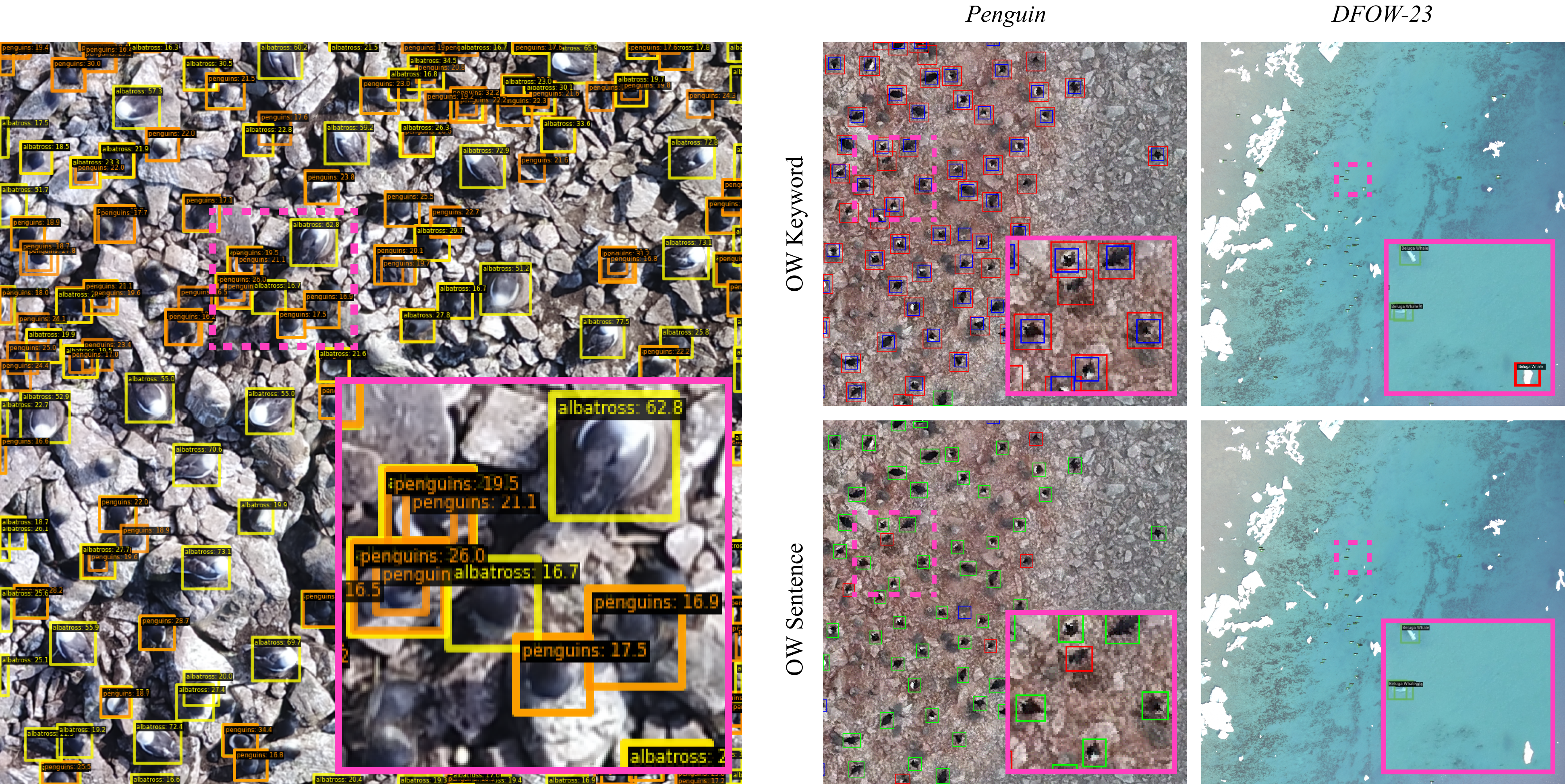
Left: multi-species detection. Right: contrasts the performance of the OW Keyword and OW Sentence models. TP is marked as green, FP as red, FN as blue. In some cases, grounding with descriptive sentences appears to improve bounding box tightness and robustness to background features.
Since our model is trained using fine-semantic captions, it developed a nuanced understanding of the world. The below figures shows the prediction of the model with different captions.
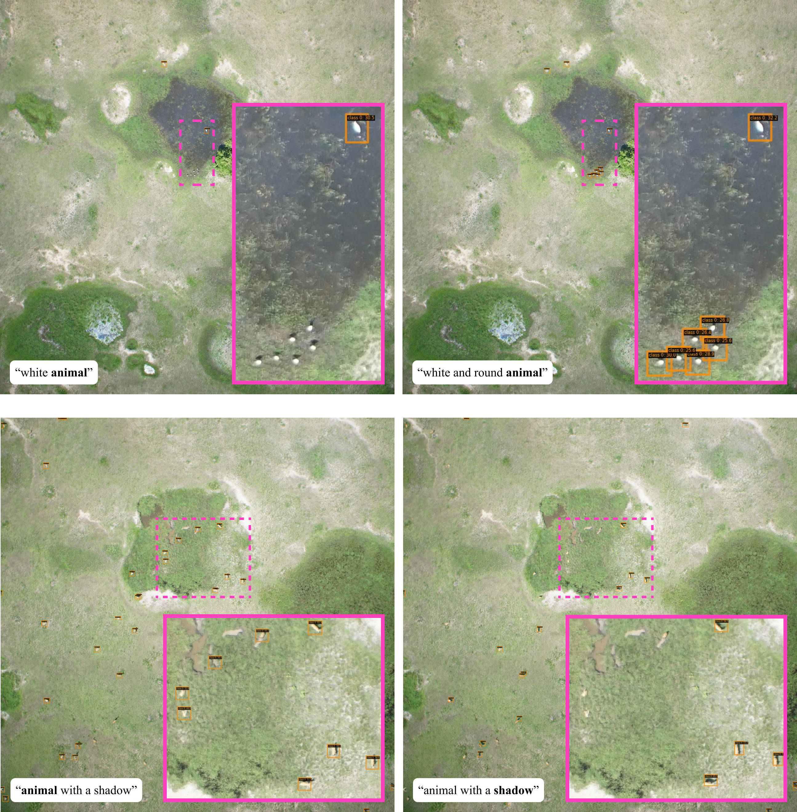
Zero-shot detection on Virunga-Garamba for different text prompts, where bolded text represents the class model was asked to predict. Our model exhibits semantic understanding of shape and shadows.
Social target Search
In the wild, animals such as lions, zebras, and whales often live in groups. Traditional aerial surveys aim to capture entire animal hotspots; however, advancements in satellite imaging resolution have made it possible to focus on smaller, targeted areas, significantly reducing costs. To capitalize on this, we propose an intelligent search strategy called Social Target Search. This method leverages the social behavior of animals and employs k-nearest neighbors and breadth-first search algorithms to selectively sample images or areas with a high probability of containing animals. The approach is using the prior information that ‘if an animal is detected in one image, there is a strong likelihood of finding more animals in neighboring images.’
Among the datasets used, only the in-house DFO whale dataset includes georeferencing. Other publicly available datasets lacked georeferencing, maybe to protect the species. To evaluate our Social Target Search method, we utilized whale survey data collected by DFO in three different years.
Below gif shows the images explored at various steps using our Social Target search method.
DFO Beluga 2014
DFO Narwhal 2016
DFO Beluga 2017
| Dataset | % Images Analyzed | % Explored Images Containing Whales | % Whales Detected |
|---|---|---|---|
| DFOW14 | 32.3 ± 11.2 | 96.3 ± 0.6 | 98.7 ± 0.4 |
| DFOW16 | 56.8 ± 14.5 | 95.0 ± 5.0 | 97.5 ± 3.0 |
| DFOW17 | 56.9 ± 8.6 | 95.2 ± 0.5 | 98.7 ± 1.0 |
Results of the STS algorithm using the ground truth annotations as predictions. From left to right, the metrics represent: the proportion of images explored relative to the total dataset size(lower percentage is preferable), the proportion of explored images containing whales relative to the total number of whale-containing images in the dataset, and the detection rate of whales.
The below figure shows the location of all the images and the particular images explored by our search algorithm.
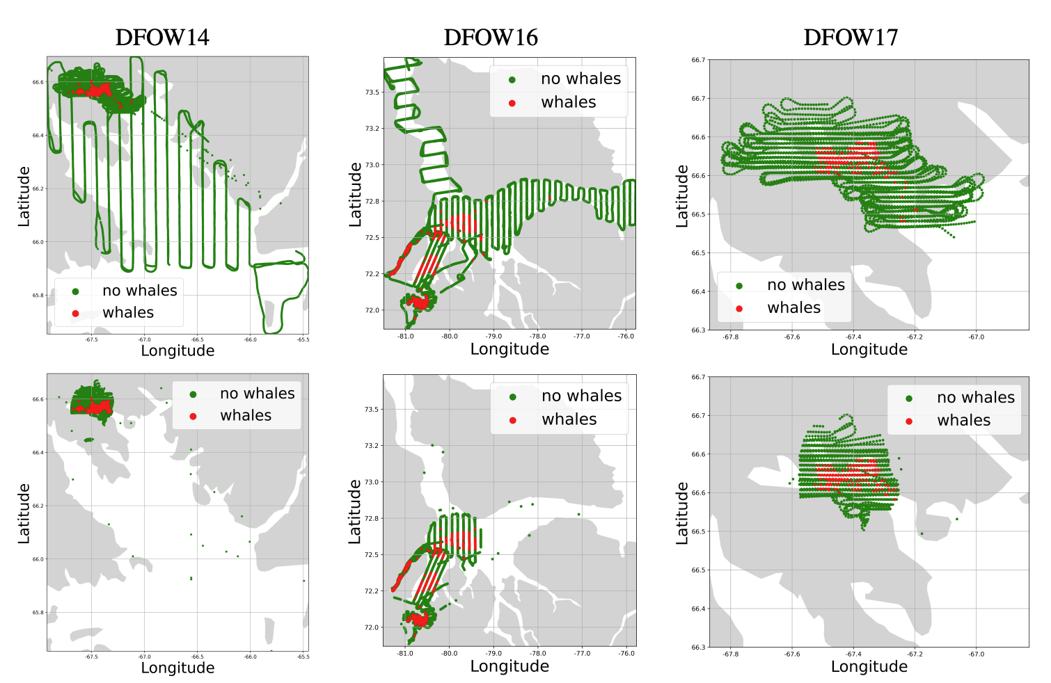
Top row: Location of all images in the datasets. Red dots indicate images with at least one annotated whale, green dots indicate images with no whales annotated. Note the clustering of whale-positive images. Bottom row: Location of the images explored by the STS algorithm. Observe the reduction in images searched.
In the results above, ground-truth annotations were used to evaluate STS. For real-world applicability, we propose using the OpenWildlife model to provide annotations for the sampled images instead of relying on ground-truth data. We did not train the OpenWildlife model on the DFO Whale 2017 dataset. Now we use OpenWildlife model with Social target search to determine the locations of whale in the entire dataset.
Below table shows the result of social target search. Our search method finds 80% of total whales while exploring only 33% of the total images.
| OW Model | % Images Analyzed | % Images Containing Whales | % Whales Detected |
|---|---|---|---|
| Sentence | 33.2 ± 5.9 | 43.2 ± 0.3 | 79.6 ± 1.2 |
| Keyword | 29.5 ± 8.1 | 38.0 ± 3.4 | 65.7 ± 3.8 |